

Fast Marching for Robust Surface Segmentation
Falko Schindler and Wolfgang Foerstner (LNCS, PIA 2011)
Contents
Download
Software available at: http://www.ipb.uni-bonn.de/html/software/fastfps/fastfps.zip
Usage example
Before detailing the following lines, we show an example of how to use the segmentation via Fast Marching Farthest Point Sampling in 5 simple steps.
1) Load a mesh:
[X, TRI] = read_off('examples/cube_6000_0-01.off');
2) Collect neighbors of each vertex:
neighbors = collectNeighborsTri(TRI);
3) Compute features, e.g. normals:
normals = computeNormals(X, neighbors, 2);
4) Select flat areas via local curvature:
curvature = arrayfun(@(i) sum(std(normals(neighbors{i}, :))), 1 : size(X, 1));
flat = curvature < median(curvature);
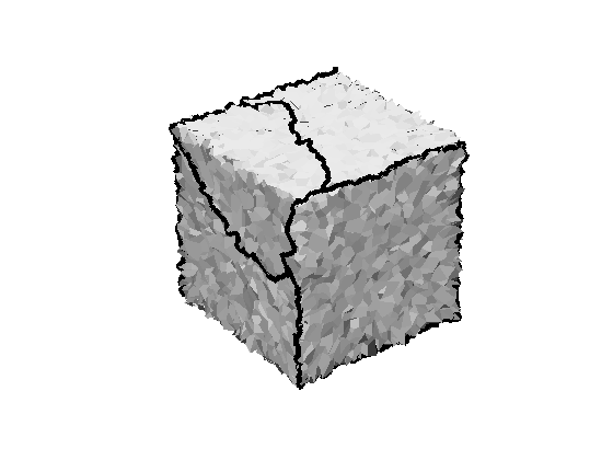
5) Perform segmentation:
label = fastfps(neighbors, normals, X, 0.01, flat);
plotMesh(1, X, TRI);
plotBoundaries(-1, X, TRI, label);
Incremental segmentation stopped at 21 segments.
Decremental segmentation stopped at 6 segments.
Minimal example in more detail
We start by loading one of the demo files in the "examples" folder. The file "cube_6000_0-001.off" is a synthetically generated cube of size 1x1x1 with 6000 vertices and Gaussian noise of sigma=0.001 for all vertex coordinates. Due to its simplicity we use the Object File Format.
[X, TRI] = read_off('examples/cube_6000_0-001.off');
With the function "collectNeighborsTri" we create a cell array with one cell for each vertex. Each cell contains indices of all neighboring vertices.
neighbors = collectNeighborsTri(TRI);
As an example for possible features we compute surface normals. The function "computeNormals" uses the previously collected neighbors of each vertex and yields the normal vector.
normals = computeNormals(X, neighbors);
With the triangular mesh represented by "neighbors" and a feature matrix "normals" we have the incredients for calling the segmentation "fastfps". We expect the cube to consist of 6 segements.
label = fastfps(neighbors, normals, 6);
Incremental segmentation stopped at 6 segments.
Decremental segmentation stopped at 6 segments.
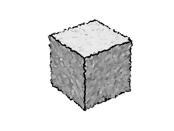
We plot the loaded mesh, given as Nx3 vertex matrix X and Tx3 triangulation TRI into figure 1. The resulting segmentation "label" is visualized using the function "plotBoundaries". The negative figure handle indicates not to clear the mesh before adding boundaries.
plotMesh(1, X, TRI);
plotBoundaries(-1, X, TRI, label);
To obtain a more intuitive result, we will introduce robust normals in the next example.
Robust surface normals
The function "computeNormals" allows to pass an additional argument indicating the degree of robustness. E.g. calling "computeNormals(..., 1)" includes neighbors of neighboring vertices when computing the normal vector. We even use neighbors of degree 2.
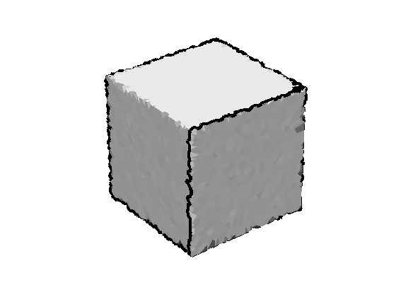
normals = computeNormals(X, neighbors, 2);
label = fastfps(neighbors, normals, 6);
plotMesh(1, X, TRI);
plotBoundaries(-1, X, TRI, label);
Incremental segmentation stopped at 6 segments.
Decremental segmentation stopped at 6 segments.
The result is still not what one would expect, but can be improved by first oversegmenting the surface and decrementally removing segments.
Incremental and decremental segmentation
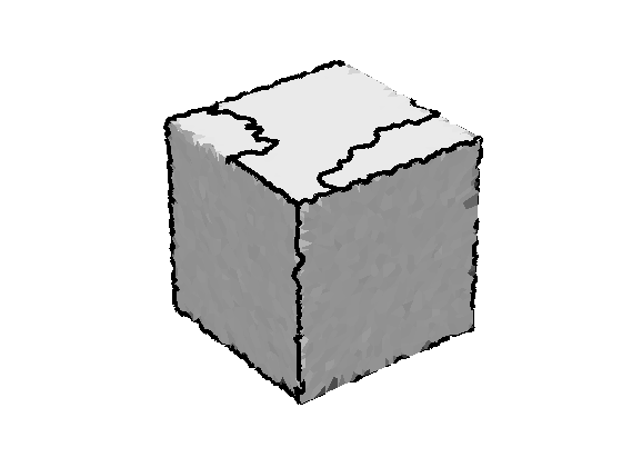
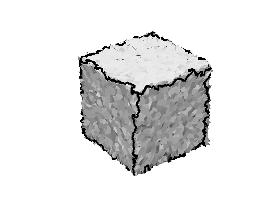
Since incrementally sampling 6 segments does not yield satisfactory results, we oversegment the cube with 20 segments before decrementally removing segments.
label = fastfps(neighbors, normals, 20, 6);
plotMesh(1, X, TRI);
plotBoundaries(-1, X, TRI, label);
Incremental segmentation stopped at 20 segments.
Decremental segmentation stopped at 6 segments.
This segmentation looks satisfactory. Now we will further increase robustness to noise by steering the sampling process to more stable areas.
Sampling on flat areas only
When working on really noisy data, segment seed points are likely to be sampled on surface edges.
[X, TRI] = read_off('examples/cube_6000_0-01.off');
neighbors = collectNeighborsTri(TRI);
normals = computeNormals(X, neighbors, 2);
label = fastfps(neighbors, normals, 6);
plotMesh(1, X, TRI);
plotBoundaries(-1, X, TRI, label);
Incremental segmentation stopped at 6 segments.
Decremental segmentation stopped at 6 segments.
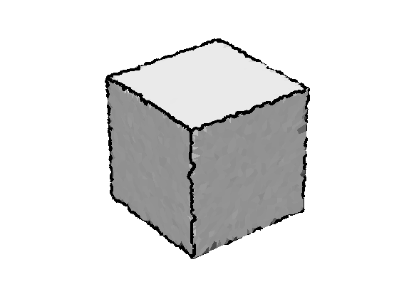
Therefore we restrict sampling seeds to flat areas only. We determine flat vertices by evaluating their curvature which is approximated by the standard deviation of neighboring normal directions.
curvature = arrayfun(@(i) sum(std(normals(neighbors{i}, :))), 1 : size(X, 1));
flat = curvature < median(curvature);
label = fastfps(neighbors, normals, 6, flat);
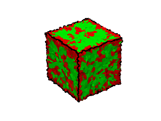
plotMesh(1, X, TRI, flat);
plotBoundaries(-1, X, TRI, label);
Incremental segmentation stopped at 6 segments.
Decremental segmentation stopped at 6 segments.
Automatic stopping criteria for piece-wise planar meshes
In case of piece-wise planar surface meshes, like the cube, we can use the automatice stopping criteria based on the segment's planarity. Therefore we need to provide vertex coordinates and their accuracy.
label = fastfps(neighbors, normals, X, 0.01, flat);
plotMesh(1, X, TRI);
plotBoundaries(-1, X, TRI, label);
Incremental segmentation stopped at 21 segments.
Decremental segmentation stopped at 6 segments.

Neighbors via k-d tree
It is also possible to obtain the topology "neighbors" using Euclidean distances and a k-d tree. This might be helpful if a triangulation is inaccessible.
addpath kdtree;
neighbors = collectNeighborsKd(X, 0.05);
normals = computeNormals(X, neighbors, 2);
curvature = arrayfun(@(i) sum(std(normals(neighbors{i}, :))), 1 : size(X, 1));
flat = curvature < median(curvature);
label = fastfps(neighbors, normals, X, 0.01, flat);
plotMesh(1, X, TRI);
plotBoundaries(-1, X, TRI, label);
Incremental segmentation stopped at 30 segments.
Decremental segmentation stopped at 6 segments.
Reference
For detailed information please refer to Schindler and Foerstner (2011):
 @inproceedings{Schindler*11:fast,
   author = {Schindler, Falko and F\"orstner, Wolfgang},
   booktitle = {LNCS, Photogrammetric Image Analysis},
   title = {{Fast Marching for Robust Surface Segmentation}},
   year = {2011}
 }