

Bundle Adjustment for Multi-camera Systems with Points at Infinity
Johannes Schneider, Falko Schindler, Thomas Laebe, and Wolfgang Foerstner (ISPRS 2012)
Contents
A. Introduction
Our recently proposed rigorous bundle adjustment BACS (Bundle Adjustment for Camera Systems) for omnidirectional and multi-view cameras enables an efficient maximum-likelihood estimation of the homogeneous scene points X_i (including points far away or at infinity) and the motion matrices M_t of the extended collinearity equation m_{ict} ~ P_c M_t^{-1} X_i by minimizing the statistical meaningfull L2-Norm of the residuals.
Line preserving cameras with known inner calibration as well as their orientation within the multi-camera system, represented by P_c, are assumed to be known. For initialization sufficiently accurate approximate values for scene point coordinates X_i and motion matrices M_t are assumed to be known.
We show how to apply our proposed bundle adjustment on the simulated parking lot scene introduced in the related paper with and without points at infinity and how to consider outliers in the observations.
Download: bacs-v0.1-matlab.zip (May 25, 2012)
B. Usage example
As a first example we show how to apply the proposed bundle adjustment on the parking lot data set without scene points at infinity.
dataset = 'parkinglot_near';
1.) Load input:
[l, Sll, ijt, Xa, Ma, P] = readinput( dataset );
(see E. Data formats for explaination of the input format of the ascii-files and the matlab variables.)
2.) Call BACS without optional arguments
If the spatial expanse of the whole blog is very large compared to the known translations in P, we give the scale a weaker influence for the definition of the gauge in Shh(7,7), which is the covariance matrix of the parameters defining the gauge.
Shh = diag( [zeros(1,6), 1e4 ] );
[ld, Xd, Md, Sdd, s0dsq, vr, w, iter] = bacs( l, ijt, Sll, Shh, Xa, Ma, P );
... Starting BACS ...
I=50 | C=3 | T=21 | N=3150
eps=1e-06 | maxIter=10 | tau=0e+00 | nearRatio=100% | k=Inf
Iter: 1 // mu = 0 // convCrit: 7e+02 // 0.00% rewighted
Iter: 2 // mu = 0 // convCrit: 1e+02 // 0.00% rewighted
Iter: 3 // mu = 0 // convCrit: 2e+00 // 0.00% rewighted
Iter: 4 // mu = 0 // convCrit: 1e-04 // 0.00% rewighted
Iter: 5 // mu = 0 // convCrit: 8e-08 // 0.00% rewighted
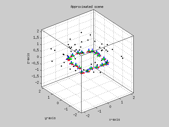
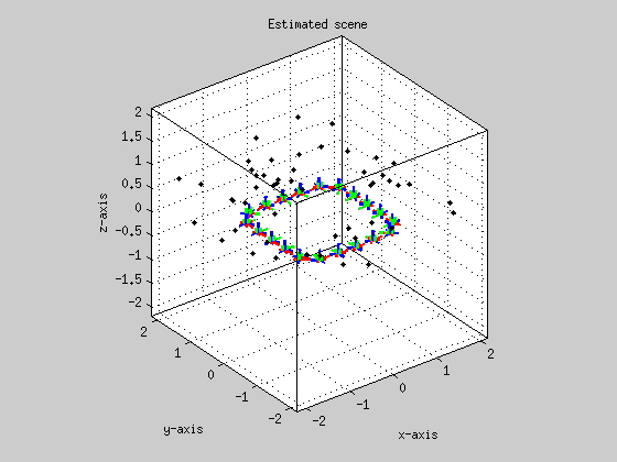
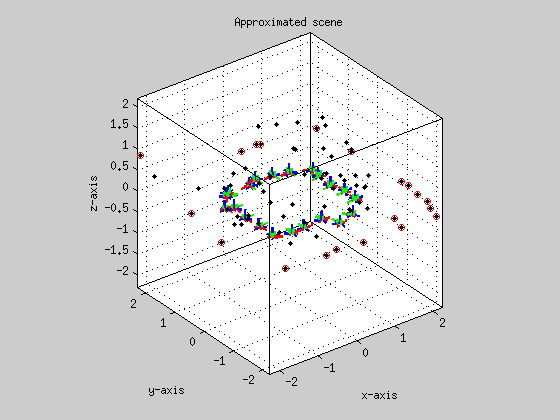
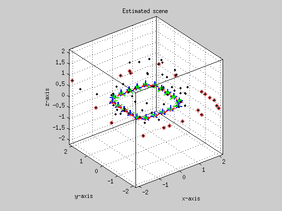
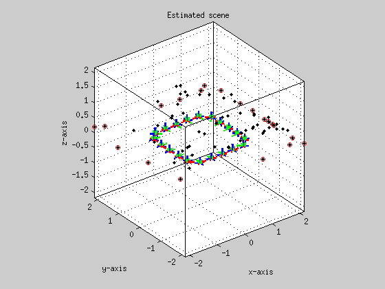
3.) Plot approximated and estimated scene (optional):
figure; hold on; grid on; box on;
plotscene( Xa, Ma, P ); title('Approximated scene');
figure; hold on; grid on; box on;
plotscene( Xd, Md, P ); title('Estimated scene');
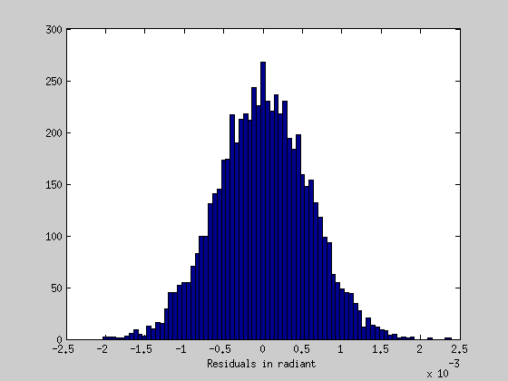
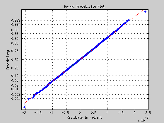
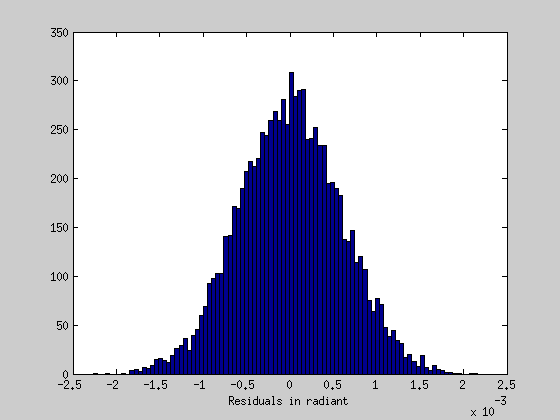
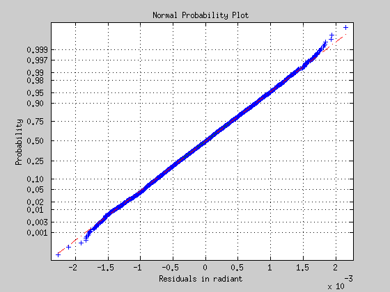
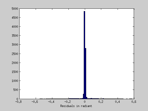
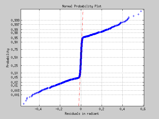
4.) Show residuals (optional):
figure; hist( vr(:), sqrt(numel(vr)) ); xlabel('Residuals in radiant');
figure; normplot( vr(:) ); xlabel('Residuals in radiant');
5.) Save estimated values / results (optional):
writeoutput( ld, Xd, Md, Sdd, vr, w, dataset );
C. Usage example with points at infinity
The following datasets contain 20 scene points at infintiy.
dataset = 'parkinglot_far';
1.) Load input:
[l, Sll, ijt, Xa, Ma, P] = readinput( dataset );
2.) Call BACS:
In the presence of scene points at infinity, we can apply the centroid constraint only on nearRatio nearest scene points.
[ld, Xd, Md, Sdd, s0dsq, vr, w, iter] = bacs( l, ijt, Sll, Shh, Xa, Ma, P, 'nearRatio', 0.5 );
... Starting BACS ...
I=70 | C=3 | T=21 | N=4410
eps=1e-06 | maxIter=10 | tau=0e+00 | nearRatio=50% | k=Inf
Iter: 1 // mu = 0 // convCrit: 3e+03 // 0.00% rewighted
Iter: 2 // mu = 0 // convCrit: 3e+02 // 0.00% rewighted
Iter: 3 // mu = 0 // convCrit: 2e+02 // 0.00% rewighted
Iter: 4 // mu = 0 // convCrit: 3e+01 // 0.00% rewighted
Iter: 5 // mu = 0 // convCrit: 5e-01 // 0.00% rewighted
Iter: 6 // mu = 0 // convCrit: 1e-04 // 0.00% rewighted
Iter: 7 // mu = 0 // convCrit: 3e-08 // 0.00% rewighted
3.) Plot approximated and estimated scene:
figure; hold on; grid on; box on;
plotscene( Xa, Ma, P ); title('Approximated scene');
figure; hold on; grid on; box on;
plotscene( Xd, Md, P ); title('Estimated scene');
4.) Show residuals:
figure; hist( vr(:), sqrt(numel(vr)) ); xlabel('Residuals in radiant');
figure; normplot( vr(:) ); xlabel('Residuals in radiant');
5.) Save estimated values:
writeoutput( ld, Xd, Md, Sdd, vr, w, dataset );
D. Usage expample with points at infinity and outliers
In the presence of outliers in the observed camera rays, we can robustify the cost function by the constant k according to Huber (1981).
dataset = 'parkinglot_outlier';
1.) Load input:
[l, Sll, ijt, Xa, Ma, P] = readinput( dataset );
2.) Call BACS:
Shh = diag( [zeros(1,6), 1e4 ] );
[ld, Xd, Md, Sdd, s0dsq, vr, w, iter] = bacs( l, ijt, Sll, Shh, Xa, Ma, P, 'nearRatio', 0.5, 'k', 3 );
... Starting BACS ...
I=70 | C=3 | T=21 | N=4410
eps=1e-06 | maxIter=10 | tau=0e+00 | nearRatio=50% | k=3.0
Iter: 1 // mu = 0 // convCrit: 7e+02 // 0.00% rewighted
Iter: 2 // mu = 0 // convCrit: 2e+02 // 19.12% rewighted
Iter: 3 // mu = 0 // convCrit: 2e+01 // 10.25% rewighted
Iter: 4 // mu = 0 // convCrit: 8e+00 // 10.05% rewighted
Iter: 5 // mu = 0 // convCrit: 3e+00 // 10.05% rewighted
Iter: 6 // mu = 0 // convCrit: 1e+00 // 10.05% rewighted
Iter: 7 // mu = 0 // convCrit: 4e-01 // 10.05% rewighted
Iter: 8 // mu = 0 // convCrit: 2e-01 // 10.05% rewighted
Iter: 9 // mu = 0 // convCrit: 6e-02 // 10.05% rewighted
Iter: 10 // mu = 0 // convCrit: 2e-02 // 10.05% rewighted
3.) Plot approximated and estimated scene:
figure; hold on; grid on; box on;
plotscene( Xa, Ma, P ); title('Approximated scene');
figure; hold on; grid on; box on;
plotscene( Xd, Md, P ); title('Estimated scene');

4.) Show residuals:
figure; hist( vr(:), sqrt(numel(vr)) ); xlabel('Residuals in radiant');
figure; normplot( vr(:) ); xlabel('Residuals in radiant');
5.) Save estimated values:
writeoutput( ld, Xd, Md, Sdd, vr, w, dataset );
E. Data formats
Input and results of the bundle adjustment can be imported and exported as ascii-files in the corresponding folders with the matlab functions readinput and writeoutput. The input files has to be placed in the relative directory input/dataset/ and the output files are stored in the relative directory output/dataset/ whereby dataset has to be defined.
Columns of the containing data have to be delimited by a comma. Every entity is arranged among the others delimited by wraped lines.
Input:
- rays.dat (Nx3): contains in each row the n=1,...,N observed camera ray vectors m_n.
- linkage.dat (Nx3): contains in each n-th row the three indices i, c and t providing the conjunction between the n-th observed camera ray which is the projection ray of i-th scene point X_i at t-th pose M_t into c-th camera P_c.
- covariances.dat (Nx6): contains covariance matrices C_n of the n-th observed camera ray m_n. Since covariance matrices are symmetric only elements of the main diagonal and upper triangle are assembled in a row with [C11, C22, C33, C12, C23, C13]_n.
- motions.dat (4Tx4): contains the t=1,...,T approximate homogeneous motion matrices M_t among each other. Each t-th motion matrix requires four rows.
- points.dat (Ix4): contains the i=1,...,I approximate homogeneous scene points X_i.
- projections.dat (3Cx4): contains the c=1,...,C projection matrices P_c among each other. Each c-th projection matrix requires three rows.
Output:
- motions.dat (4Tx4): contains the t=1,...,T estimated homogeneous motion matrices M_t among each other. Each t-th motion matrix requires four rows.
- points.dat (Ix4): contains the i=1,...,I estimated homogeneous scene points X_i.
- rays.dat (Nx3): contains in each row the n=1,...,N estimated camera ray vectors m_n.
- corrections.dat (Nx2): contains the n=1,...,N estimated corrections v_n of the observed camera rays in minimal representation.
- motioncovariance.dat (6Tx6T): full covariance matrix of the estimated rotation and translation parameters at every time instance t=1,...T. Three rotations are followed by three translations for each time instace t.
F. Reference
For detailed information please refer to Schneider et al. (2012)
 @inproceedings{schneider*12:bundle,
   author = {Schneider, Johannes and Schindler, Falko and L\"aebe, Thomas and F\"oerstner, Wolfgang},
   booktitle = {22nd Congress of the International Society for Photogrammetry and Remote Sensing (ISPRS)},
   title = {{Bundle Adjustment for Multi-camera Systems with Points at Infinity}},
   year = {2012}
   note = {to appear}
 }
Do not hesistate to contact us in case you have any questions.